Contents
stationary BD for sloc
path('/home/hu/path/p2p2/p2plib',path);path('../p2poclib',path);
Scenario 1, FSC/FSI branch
close all; p=[];lx=2*pi/0.44; ly=0.1; nx=50; ny=1; sw=1;
p=slinit(p,lx,ly,nx,ny,sw); p=setfn(p,'f1'); screenlayout(p);
first res=8.73997e-15
Problem directory name: f1
find bif.points from FSC/FSI branch
p.nc.nsteps=100; p=cont(p);
step lambda      y-axis    residual iter meth   ds
   0 got first point with lam=0.55, res=8.73997e-15
   - now lam=0.56
   1 got second point with lam=0.56, res=4.29448e-13
   2    0.56214    0.85109 8.09e-15    2  arc    0.10000
   3    0.56648    0.86066 7.56e-09    1  arc    0.20000
   4    0.57547    0.88090 5.13e-14    2  arc    0.40000
   5    0.58486    0.90276 8.92e-14    2  arc    0.40000
   6    0.59469    0.92649 1.66e-13    2  arc    0.40000
   7    0.60000    0.93971 6.39e-10    1  nat   -0.18916
   8    0.60498    0.95238 3.25e-13    2  arc    0.40000
   9    0.61576    0.98081 6.76e-13    2  arc    0.40000
  10    0.62706    1.01225 1.49e-12    2  arc    0.40000
  11    0.63888    1.04732 3.51e-12    2  arc    0.40000
  12    0.65000    1.08268 4.08e-11    1  nat   -0.03976
  13    0.65126    1.08685 9.06e-12    2  arc    0.40000
  14    0.66416    1.13203 2.62e-11    2  arc    0.40000
  15    0.67756    1.18460 8.90e-11    2  arc    0.40000
  16    0.69131    1.24731 3.83e-10    2  arc    0.40000
  17    0.70000    1.29384 6.98e-12    2  nat   -0.15035
...

FSM branch
sw=2; p=slinit(p,lx,ly,nx,ny,sw); p=setfn(p,'f2');
p.nc.dsmax=0.2; p.sol.ds=0.1; p=cont(p,25);
first res=4.5601e-09
Problem directory name: f2
step lambda      y-axis    residual iter meth   ds
   0 got first point with lam=0.55, res=4.5601e-09
   - now lam=0.56
   1 got second point with lam=0.56, res=1.07197e-09
   2    0.56894    4.03189 8.84e-09    1  arc    0.10000
   3    0.57827    3.95535 2.02e-09    1  arc    0.10000
   4    0.58799    3.87780 2.08e-09    1  arc    0.10000
   5    0.59814    3.79931 2.06e-09    1  arc    0.10000
   6    0.60000    3.78514 2.57e-09    1  nat   -0.08066
   7    0.60872    3.71996 1.95e-09    1  arc    0.10000
   8    0.61976    3.63988 1.68e-09    1  arc    0.10000
   9    0.63126    3.55929 1.18e-09    1  arc    0.10000
  10    0.64324    3.47848 3.89e-10    1  arc    0.10000
  11    0.65000    3.43430 1.17e-10    1  nat   -0.04492
  12    0.65570    3.39783 9.37e-10    1  arc    0.10000
  13    0.66862    3.31789 2.81e-09    1  arc    0.10000
  14    0.68198    3.23932 6.83e-09    1  arc    0.10000
  15    0.69573    3.16291 7.20e-14    2  arc    0.10000
...

bifurcations from f1
p=swibra('f1','bpt1','p1',-0.05); p.nc.dsmax=0.3; p=cont(p,150);
p=swibra('f1','bpt2','p2',-0.05); p.nc.dsmax=0.3; p=cont(p,150);
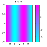
p=swibra('f1','bpt3','p3',0.05); p.nc.dsmax=0.3; p=cont(p,150);
lambda=0.727148, zero eigenvalue is 3.82343e-06
al0=-0.00498673, a1=3.06361e-06, b1=37.061, al1b=-74.1221
Problem directory name: p1
step lambda      y-axis    residual iter meth   ds
   1    0.72681    1.61793 9.77e-10    3  arc   -0.05000
   2    0.72610    1.60696 3.31e-10    2  arc   -0.05000
   3    0.72403    1.58566 1.45e-09    2  arc   -0.10000
   4    0.71852    1.55216 8.76e-14    3  arc   -0.20000
   5    0.71218    1.52895 2.44e-09    2  arc   -0.20000
   6    0.70549    1.51344 4.09e-10    2  arc   -0.20000
   7    0.70000    1.50554 1.91e-09    1  nat    0.03937
   8    0.69865    1.50416 1.20e-10    2  arc   -0.20000
   9    0.69179    1.50025 5.16e-11    2  arc   -0.20000
  10    0.68499    1.50119 6.21e-11    2  arc   -0.20000
  11    0.67828    1.50671 7.93e-11    2  arc   -0.20000
  12    0.67171    1.51674 1.29e-10    2  arc   -0.20000
  13    0.66530    1.53137 2.82e-10    2  arc   -0.20000
  14    0.65909    1.55092 8.30e-10    2  arc   -0.20000
  15    0.65313    1.57594 3.34e-09    2  arc   -0.20000
  16    0.65000    1.59216 1.16e-10    2  nat    0.09328
...
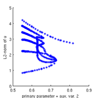
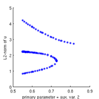
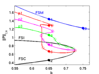
plotting of BD, L2 over b
figure(3); clf; pcmp=3; ms=5;
plotbraf('f1','bpt1',3,pcmp,'ms',ms,'lab',12,'cl','k');
plotbraf('f1','pt74',3,pcmp,'ms',ms,'fp',15,'cl','k','lt','.', 'lab',36);
plotbraf('f2','pt25',3,pcmp,'ms',ms,'lab',[11 20],'cl','b','lp',23);
plotbraf('p1','pt135',3,pcmp,'ms',ms,'cl','r','lab',[16 71]);
plotbraf('p2','pt128',3,pcmp,'ms',ms,'cl','m','lab',18);
plotbraf('p3','pt111',3,pcmp,'ms',ms,'cl','g','lab',19);
xlabel('b'); ylabel('||P||_{2,a}');
text(0.61,1.6,'FSM','color','b','fontsize',16);text(0.56,1.59,'p1','color','r','fontsize',16);
text(0.56,1.45,'p2','color','m','fontsize',16);text(0.56,1.28,'p3','color','g','fontsize',16);
text(0.56,1,'FSI','color','k','fontsize',16);text(0.56,0.5,'FSC','color','k','fontsize',16);
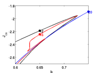
JC over b
figure(3); clf; pcmp=4; ms=0;
plotbraf('f1','bpt1',3,pcmp,'ms',ms,'cl','k', 'lab',12);
plotbraf('f1','pt74',3,pcmp,'ms',ms,'fp',22,'cl','k','lt','.');
plotbraf('f2','pt25',3,pcmp,'ms',ms,'cl','b','lab',20);
plotbraf('p1','pt135',3,pcmp,'ms',ms,'cl','r','lab',16);
xlabel('b'); ylabel('J_{ca}'); axis([0.6 0.75 -2.7 -1.8])
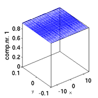
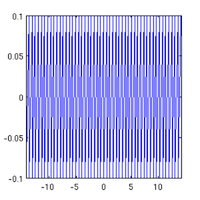
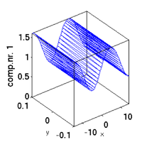
solution plotting
plot1Df('p1','pt16',1,1,1,2); pause; plot1Df('p1','pt71',1,1,1,2); pause
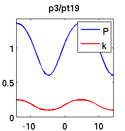
plot1Df('p2','pt18',1,1,1,2); pause; plot1Df('p3','pt19',1,1,1,2);
lam=0.65
lam=0.65
lam=0.65
lam=0.65
print CSS characteristics (for tables)
stancssvalf('p1','pt16');
p1/pt16, lam=0.65, (<u1>,<k>,jca)=(0.61 & 0.14 & -74.83)